Unsupervised Stock Market Features Construction using Bidirectional Generative Adversarial Networks(BiGAN)

Deep Learning constructs features using only raw data. The learned representation of the data outperforms expert features for many modalities including Radio Frequency (Convolutional Radio Modulation Recognition Networks), computer vision (Convolutional Deep Belief Networks for Scalable Unsupervised Learning of Hierarchical Representations) and audio classification (Unsupervised feature learning for audio classification using convolutional deep belief networks).

GAN

In the case of Convolutional Neural Networks (CNN), the data representation is learned in a supervised fashion with respect to a task such as classification. GANs learn features in an unsupervised fashion. The competitive learning process for GANs results in more of the possible feature space being explored. This reduces the potential for features being overfitted to the training data. Since the features are constructed in an unsupervised process classification algorithms trained on the features will generalize on a smaller amount of data. In fact, GANs promote generalization beyond the training data.

For a full review of GANs reference the paper Generative Adversarial Nets and tutorial for implementing a basic GAN Generative Adversarial Nets in TensorFlow.

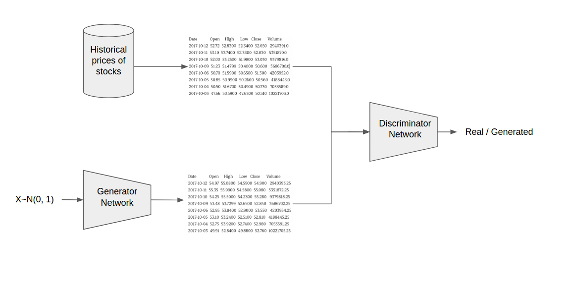
The Generator is trained to generate data that looks like historical price data of the target stocks over a distribution. The Discriminator is trained to tell the difference between the data from the Generator and the real data. The loss from the Discriminator (how the Discriminator has learned to tell if a sample in real or fake) is used to train the Generator to defeat the Discriminator. The competition between the Generator and the Discriminator forces the Discriminator to distinguish random from real variability while the Generator learns to map a distribution into the sample space.
This project explores Bidirectional Generative Adversarial Networks(BiGANs) based on the paper Adversarial Feature Learning. The primary difference in the BiGAN the Discriminator learns to determine the joint probability P(X, Z) = real/fake (where X is the sample and Z is the generating distribution). This, in turn, means that the Generator learns to encode a real sample into its generating distribution.

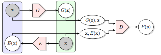
Figure from Adversarial Feature Learning

This project makes a modification to the BiGAN. Rather than learning to encode a real sample into the generating distribution,the model learns to encode the features learned by the Discriminator (rather then the raw data) into the generating distribution. For historical stock data, this architecture outperformed the BiGAN architecture.

Approach

Data Historical prices of stocks are likely not very predictive of the future price, but it is free data.

Training The GAN is trained on 96 stocks off the Nasdaq. Each stock is normalized using a 20-day rolling window (data-mean)/(max-min). The last 2 years (504 days) of trading are held out as a test set. Time series of 20 day periods are constructed and used as input to the GAN. Once the GAN is finished training, the learned encoding for the Discriminator features to the generation distribution is used as the new representation of the data. The features are not guaranteed to be predictive of the direction of the stock market, but for other modalities, they have been shown to work well. Random Forests is trained to classify whether the stock will gain 10% over the next 10 trading days. This creates an unbalanced training set so the majority class is undersampled before training the Random Forest.

Results First, let’s visualize the features learned by the BiGAN. TSNE will be used to reduce the dimensions to 2D.

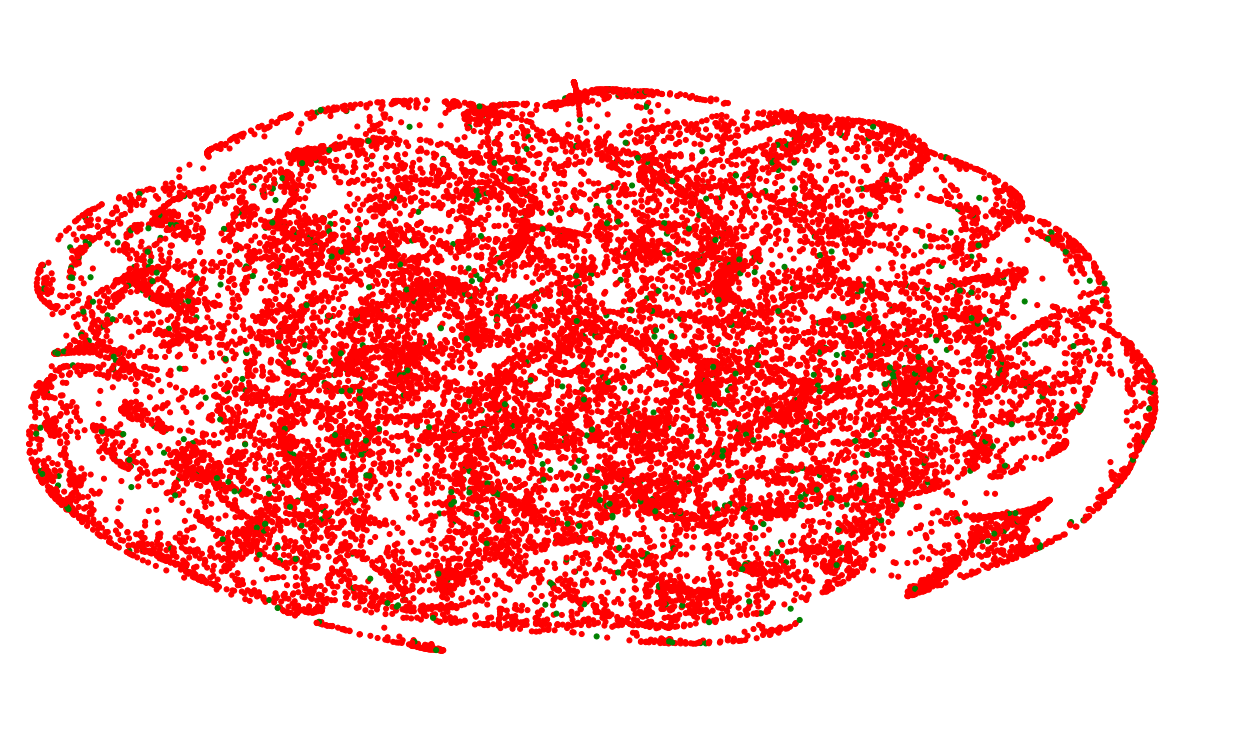
The red dots are negative samples and green are positive samples. There appears to be some structure to the features learned by the BiGAN, but not related to the target. More experimentation is needed to see what the structure is following, but I suspect the each curve is a specific stock.

Since the classes are unbalanced, due to many stocks not gaining 10% in 10 days, accuracy is a poor metric. If we always predicted that stocks would not go up then the accuracy would be above 90%. So instead of accuracy, we will use Area Under the Curve (AUC). Check out this video to learn more about AUC. An AUC of 1 would be a perfect model while an AUC of 0.5 means that the model performs the same as picking a label randomly. We can visualize the performance of the classifier using a ROC curve.

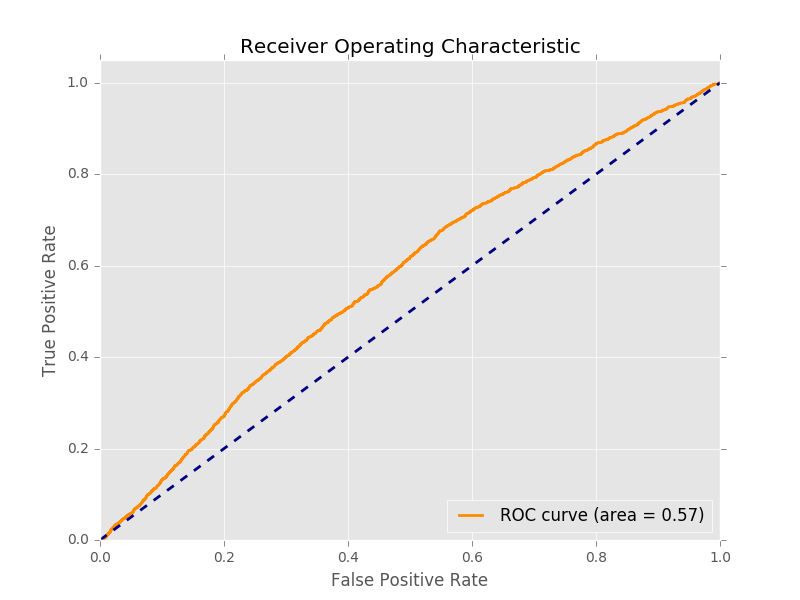
This shows that the classifier is only a little better than random. Another way of visualizing the performance of the classification algorithm is a confusion matrix.

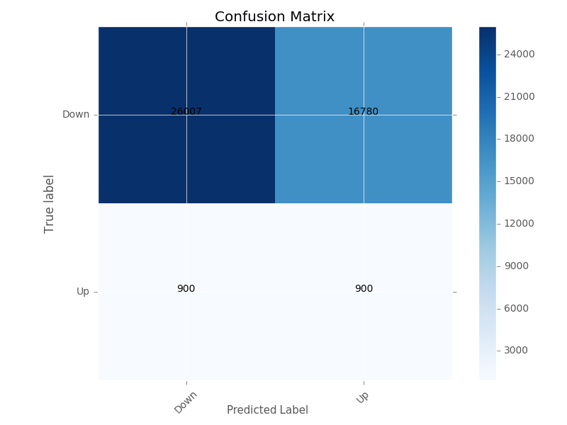
The top row shows that the classifier correctly classified 29,007 samples as true negatives while misclassifying 16,780 samples as false positives. The bottom row shows that the classifier misclassified 900 samples as false negatives and correctly classified 900 examples as true positives. The perfect confusion matrix would only have values on the diagonal.

There are a very large number of false positives. If the false positive predictions make some money (just not 10%) this could still be a valid trading strategy. So let’s look at the distribution of the percent returns from the false positive predictions.

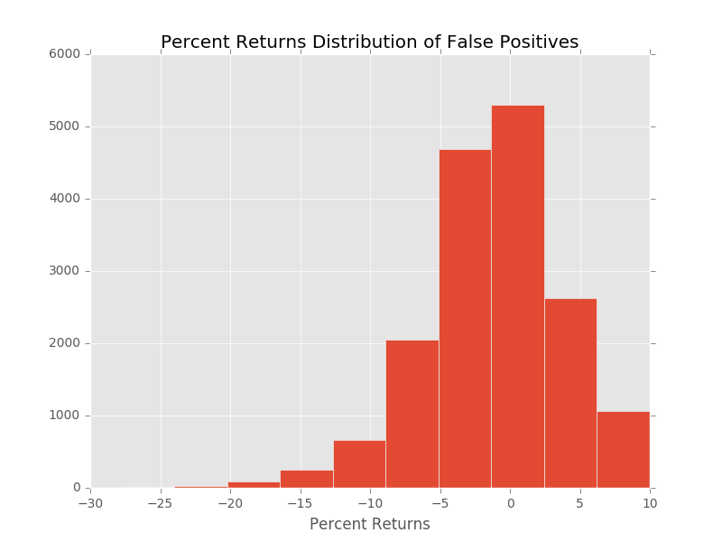
The distribution of the returns on the false positive predictions does not look promising. They appeared skewed toward negative returns.

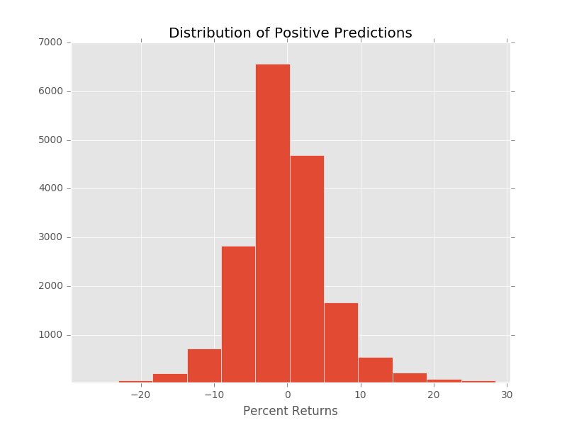
If we look at the overall distribution of the returns of all positive predictions, it still is skewed toward negative returns. The mean return for all positive predictions ends up being -0.18% a small negitive return.

After some analysis of the predictions, it appears that the model will almost always predict that a stock coming into earnings is going to gain. This is likely due to the sampling technique. The majority of the samples of a stock gaining 10% in 10 days surrounds the earnings calls. Since the data is undersampled the vast majority of the earnings calls given to the Random Forests model are earnings calls that gained 10% over the proceeding 10 days, biasing the model to predict that all earnings calls will make 10%. Possibly using a different sampling technique could solve this, such as oversampling stocks that performed badly over 10 days. It is interesting that the model can identify when an earnings call is approaching just based on the BiGAN features learned from Open, High, Low, Close and Volume.

Additional improvement should be made to the model. Currently, missing days are not explicitly taken into account. The model was tested using linear interpolation over missing days including weekends, but that hurt the overall performance of the model. It might be better to only interpolate over missing trading days rather than weekend and holidays.